📘 👨‍💻 📄 📊 R Code Templates for Use with Quarto

programming

Quarto

article

Quarto allows the direct execution of R code blocks in .qmd files. This makes it possible to generate dynamic reports, plots, statistical analyses, and interactive visualizations, all integrated with text.

Author

Blog do Marcellini

Published

June 29, 2025

← Back to the Programming Reading Guide 👨‍💻

← Back to the R Section 📊

← Back to the Programming Section 👨‍💻

1 📘 👨‍💻 📄 📊 R Code Templates for Use with Quarto

1.1 Introduction

Quarto allows the direct execution of R code blocks in .qmd files.
This makes it possible to generate dynamic reports, plots, statistical analyses, and interactive visualizations, all integrated with text.

The snippet below is the YAML header of the .qmd document, which defines the title, author, date, output format, and execution options for R code:

---
title: "R Code Templates for Use with Quarto"
author: "Blog do Marcellini"
date: 2025-06-23
format: html
editor: visual
lang: en
execute:
  engine: knitr
  echo: true
  warning: false
  message: false
---

1.2 Simple R code block

x <- 1:10
y <- x^2
y

 [1]   1   4   9  16  25  36  49  64  81 100

1.3 Creating a base plot

plot(x, y, type = "b", col = "blue", main = "Plot of x²", xlab = "x", ylab = "y = x²")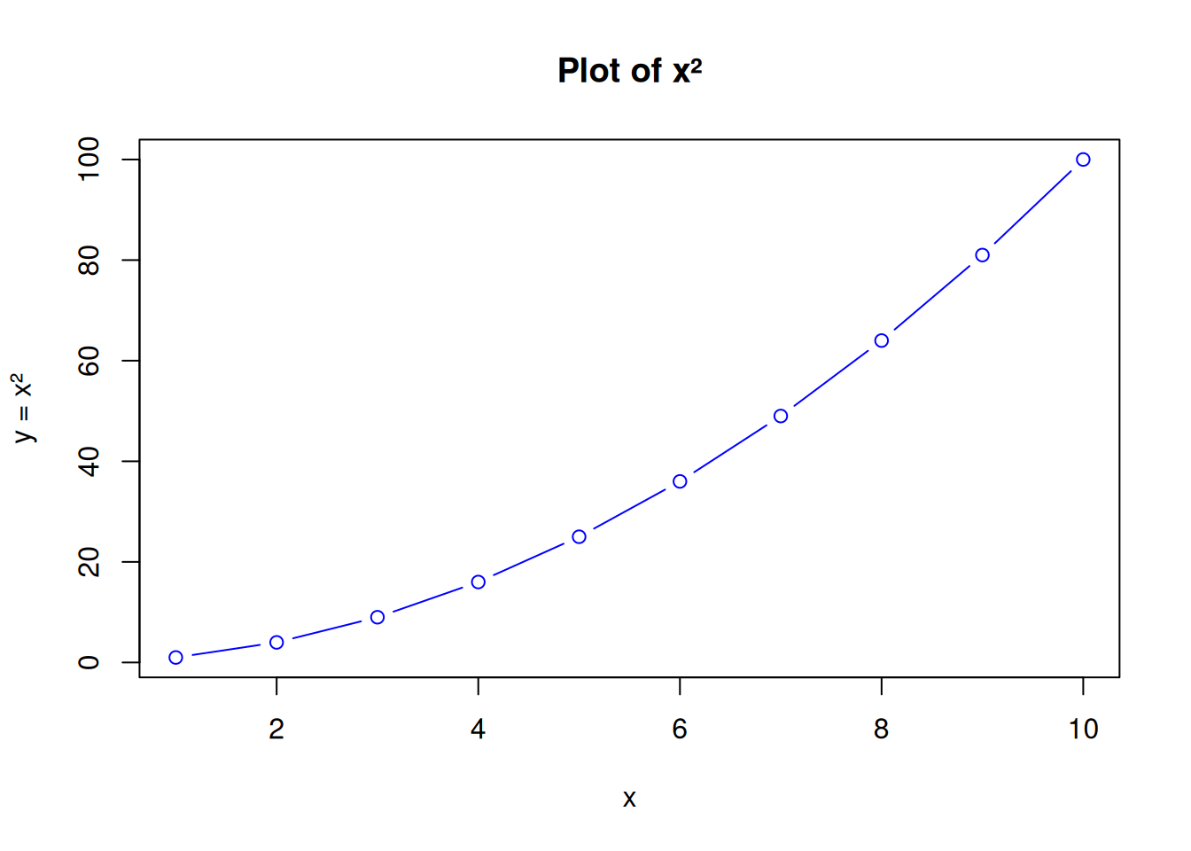

1.4 Using ggplot2

library(ggplot2)

df <- data.frame(x = x, y = y)

ggplot(df, aes(x, y)) +
  geom_line(color = "red", size = 1.2) +
  geom_point(color = "blue") +
  labs(title = "Plot with ggplot2", x = "x", y = "x²")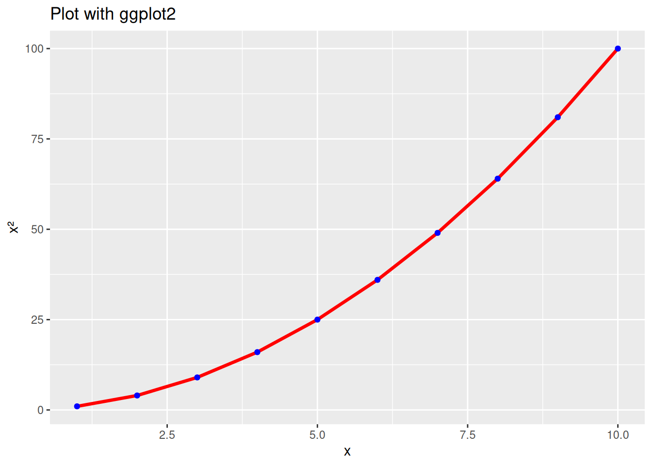

1.5 Descriptive statistics

summary(mtcars)

      mpg             cyl             disp             hp       
 Min.   :10.40   Min.   :4.000   Min.   : 71.1   Min.   : 52.0  
 1st Qu.:15.43   1st Qu.:4.000   1st Qu.:120.8   1st Qu.: 96.5  
 Median :19.20   Median :6.000   Median :196.3   Median :123.0  
 Mean   :20.09   Mean   :6.188   Mean   :230.7   Mean   :146.7  
 3rd Qu.:22.80   3rd Qu.:8.000   3rd Qu.:326.0   3rd Qu.:180.0  
 Max.   :33.90   Max.   :8.000   Max.   :472.0   Max.   :335.0  
      drat             wt             qsec             vs        
 Min.   :2.760   Min.   :1.513   Min.   :14.50   Min.   :0.0000  
 1st Qu.:3.080   1st Qu.:2.581   1st Qu.:16.89   1st Qu.:0.0000  
 Median :3.695   Median :3.325   Median :17.71   Median :0.0000  
 Mean   :3.597   Mean   :3.217   Mean   :17.85   Mean   :0.4375  
 3rd Qu.:3.920   3rd Qu.:3.610   3rd Qu.:18.90   3rd Qu.:1.0000  
 Max.   :4.930   Max.   :5.424   Max.   :22.90   Max.   :1.0000  
       am              gear            carb      
 Min.   :0.0000   Min.   :3.000   Min.   :1.000  
 1st Qu.:0.0000   1st Qu.:3.000   1st Qu.:2.000  
 Median :0.0000   Median :4.000   Median :2.000  
 Mean   :0.4062   Mean   :3.688   Mean   :2.812  
 3rd Qu.:1.0000   3rd Qu.:4.000   3rd Qu.:4.000  
 Max.   :1.0000   Max.   :5.000   Max.   :8.000

1.6 Histogram

hist(mtcars$mpg, col = "lightblue", main = "MPG Distribution", xlab = "Miles per gallon")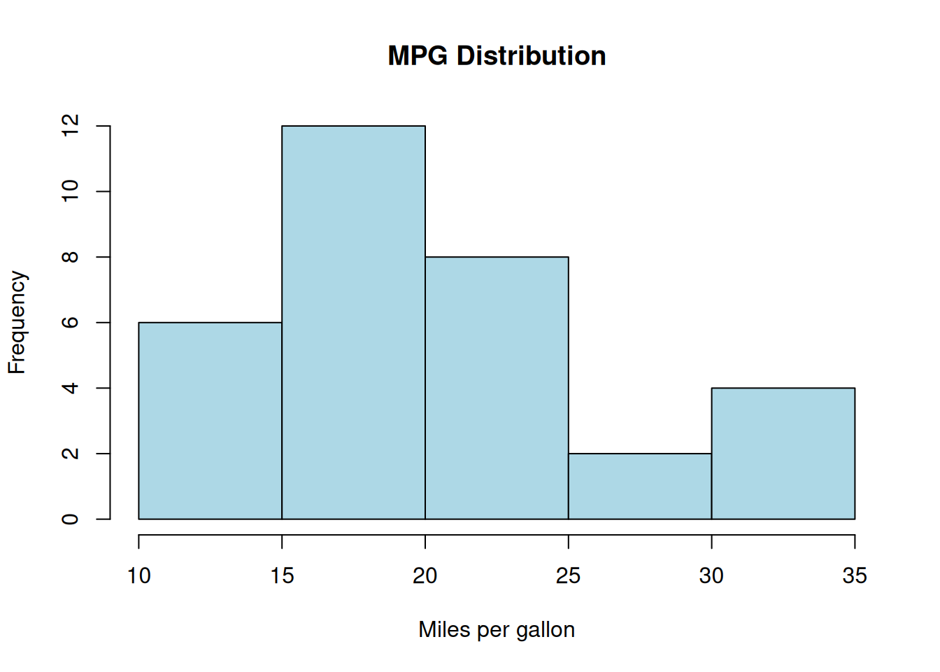

1.7 Linear simple regression

model <- lm(mpg ~ hp, data = mtcars)
summary(model)


Call:
lm(formula = mpg ~ hp, data = mtcars)

Residuals:
    Min      1Q  Median      3Q     Max 
-5.7121 -2.1122 -0.8854  1.5819  8.2360 

Coefficients:
            Estimate Std. Error t value Pr(>|t|)    
(Intercept) 30.09886    1.63392  18.421  < 2e-16 ***
hp          -0.06823    0.01012  -6.742 1.79e-07 ***
---
Signif. codes:  0 '***' 0.001 '**' 0.01 '*' 0.05 '.' 0.1 ' ' 1

Residual standard error: 3.863 on 30 degrees of freedom
Multiple R-squared:  0.6024,    Adjusted R-squared:  0.5892 
F-statistic: 45.46 on 1 and 30 DF,  p-value: 1.788e-07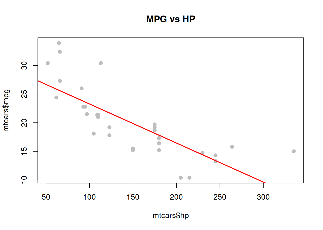

1.8 Plot with regression line

plot(mtcars$hp, mtcars$mpg, pch = 19, col = "gray", main = "MPG vs HP")
abline(model, col = "red", lwd = 2)

1.9 Formated table with knitr::kable

library(knitr)
kable(head(mtcars), caption = "First rows of the mtcars dataset")

First rows of the mtcars dataset
	mpg	cyl	disp	hp	drat	wt	qsec	vs	am	gear	carb
Mazda RX4	21.0	6	160	110	3.90	2.620	16.46	0	1	4	4
Mazda RX4 Wag	21.0	6	160	110	3.90	2.875	17.02	0	1	4	4
Datsun 710	22.8	4	108	93	3.85	2.320	18.61	1	1	4	1
Hornet 4 Drive	21.4	6	258	110	3.08	3.215	19.44	1	0	3	1
Hornet Sportabout	18.7	8	360	175	3.15	3.440	17.02	0	0	3	2
Valiant	18.1	6	225	105	2.76	3.460	20.22	1	0	3	1

1.10 Conditional results with `if`

valor <- mean(mtcars$mpg)

if (valor > 20) {
  print("The average MPG is high.")
} else {
  print("The average MPG is low.")
}

[1] "The average MPG is high."

1.11 Conclusion

With Quarto and R, it is possible to integrate text, code, and results into a single dynamic and reproducible document.
These templates are a starting point for creating statistical and scientific reports with a high professional standard.

← Back to the Programming Reading Guide 👨‍💻

← Back to the R Section 📊

← Back to the Programming Section 👨‍💻

🔝 Back to Top

Blog do Marcellini — Exploring Mathematics, Statistics, and Physics with Rigor and Beauty.